— Why you dive computer is not always right.
A model may mean different things. It can signify a miniaturisation, like the kit airplanes some of us assembled when we were kids or an electrical model railway. It can mean mimicking or resembling something, the appearance or behaviour of which we want to emulate or replicate—what is also known as a simulation. Furthermore, it may also stand for simplification. In the framework of this article, all of these meanings will apply to some extent.

Contributed by
We resort to models when we need to simplify complex mechanisms or relationships in order to make decisions, predict the outcome of some processes, or analyse consequences of some decisions—sometimes with the aid of computers running complex simulations of various scenarios.
In fields related to diving, models are predominantly used in ecology and hyperbaric physiology - and in dive computers.
Climate change, the effects of which is another recurring topic in this publication, is also analysed by running complex models.
Representations
The compartments or “tissues” used in decompression algorithms in dive computers are, for example, not real tissues but fictional representations with a simulated behaviour, which has been designed to resemble the on and off gassing that takes place inside and between the real tissues making up the organism of a diver.
In order to make these calculations manageable, a number of simplifications and assumptions have to be made. The truth is that nobody knows exactly what goes on at the microscopic level, the dynamics of which are still up for much discussion and a subject of ongoing research.
Close enough
The models (or mathematical representations) used in dive computers make predictions, which correlate closely enough with actual data and observations made during tests conducted by hyperbaric researchers over many decades. We use and trust these instruments to keep us out of harm’s way.
For the most part, they do—many thousands of dives have been conducted safely and without any incidences.
However, a substantial proportion of occurrences of decompression illness (DCI) has happened to divers who stayed well within the limits and without any immediate explanation.
It is a testament to the fact that dive computers, no matter how sophisticated they may have otherwise become over time, are not able to state what is actually going on in the body—only what is, in all likelihood, going on.
They are simply predictors. Until some fancy technology comes around which can directly monitor gas loading in various tissues in real time as we dive, it is all they can do.
Why can’t models be accurate?
In order to better illustrate the limitations of models, let us look into how models are used elsewhere, say, in aquatic ecology—a field that should also have plenty of relevance to divers.
Researchers and managers would typically like to know how an ecosystem behaves, or about its resilience to the impact of various human activities. It could be a matter of water quality, management of fisheries (such as setting sustainable quotas), the effect of marine protected areas, the effect of some major infrastructure (such as a bridge or dam), or the restoration of lakes, wetlands or seas.
In other words, models are about describing various changes to the overall system, along with the relative magnitude and significance of its constituent processes. In doing so, the most important processes and factors are prioritised, as it is an understanding of the general behaviour of the system, and usually not the finer details, which is sought.
Models are very much about flows (i.e. of matter or energy) between compartments. For example gasses that moves between simulated human tissues or how carbon would flow through an ecosystem. Let’s take a look at the mechanics.
Back to school
We can use a familiar elementary-school math example to demonstrate how flows are calculated:
Ben travels in a car between city A and town B, which are 100km apart, and he is driving at an average velocity of 50kph. Most of us can easily figure out, without the use of a calculator, that it would take Ben two hours to get from A to B, or that in 30 minutes, he would have travelled 25km, and so on.
Such calculations are trivial, and we perform them every time we leave the house to be somewhere else on time.
In a model, the two towns are the compartments and the car is the matter that “flows” between them at a certain rate (its velocity). Timetables can be viewed as simple models. They predict with reasonable accuracy when a bus or train is going to make it to its destination, under the presumption that there are no major accidents holding us up.
We will get back to the importance of underlying assumptions in a moment, but if we leave extraordinary circumstances out of the picture for now, we do not need to precisely account for the effect of every traffic light or the number of potholes in the road along the route as these effects usually do not make a major difference in the end.
The above example assumes an average or even speed, an assumption or condition which is important to keep in mind going forward.
Dynamic systems
What if the speed was not even but fluctuated significantly? Say, if the subject (or “compartment,” in model-speak) we are looking at is not a car or a bus travelling predictably along a road, but rather some volume of water flowing in the ocean, subject to tides and wind, passing through a strait or tumbling down a river?
The systems’ behaviours we want to analyse—perhaps for the sake of making some forecast—are often highly dynamic, and the systems’ constituent compartments can be simultaneously affected by many factors.
Complex systems may even exhibit chaotic behaviours on various levels, such as weather, but let’s ignore that complication for the time being.
Describing system dynamics
In order to understand the dynamics of systems and how they are described mathematically, we can stick with example of the car going from A to B and take a closer look at the relationship between location, velocity and acceleration:
Velocity (v) is the rate at which you change location and acceleration (a) is the rate at which you change your velocity. Or more formally (where Δ means the difference or change):
These parameters are interlinked in a way so if you know your acceleration you can also calculate your speed and time of arrival and vice versa.
From our physics classes, we may recall the classical law of motion as expressed in the following equation:
p = p0 + vt + ½ at2
In this equation, p is the position of the moving object, p0 is the starting position, v is velocity, t is time and a is acceleration. In terms of an everyday commute, it simply means that:
Your current location = Starting point
+ (speed x travel time)
+ ½ (acceleration x time2)
If we sketch out such a typical commute on a graph (Figure 2), it should become apparent that the process of driving from A to B is the sum of three constituent processes; You set out by accelerating up to your cruising speed, coast along at a steady pace, and then decelerate at the end as you come to a stop.
Figure 2. Graph of a typical commute in a car, driving from A to B. The areas under the curve (a + b + c) is the distance covered. Acceleration is change of speed. The slope of the graph shows acceleration (+/-), which in this case, is always linear (even) as the lines are straight.
The speed changes only in the beginning and the end of the journey, so this process of changing your location is fairly simple to calculate. In fact, the distance travelled is simply the area under the curve. In this case, we just have to add up the three areas a, b and c.
In this simplified case, acceleration is always constant, corresponding to the slope of the curve, which comprises straight lines. First, it has a positive but constant value; then, zero; and finally, it has a negative value, as the car is coming to a stop.
All we have to do in order to calculate the distance covered is add up the area of the two triangles and the rectangle.
When processes fluctuate
But what if the process was far more uneven and the changes (in this case, in velocity) represented a complex curve?
Say, if the car would constantly speed up and brake? The next figure (right) shows an example where speed fluctuates—the slope of the gradient is the acceleration/deceleration.
Then, simple geometry or linear algebra would not be able to provide an immediate answer, and we would have to resort to integral calculus to precisely calculate the area under the curve, such as the yellow area on the curve below. (For those not familiar with integral calculus, you may think of it as summing up the areas of many infinitesimally thin vertical rectangles that can fit into the yellow area in Figure 3).
Figure 3. Example of a velocity vs. time graph, showing the relationship between (a changing) velocity v on the Y-axis, acceleration a (the three green tangent lines represent the values for acceleration at different points along the curve), and distance travelled s (the yellow area under the curve). Source: Wikipedia
This is all fine and dandy if it is possible to integrate the equation describing the motion—which, in the overall context of this article, should just be viewed as a stand-in, also representing processes in biology and physiology.
The big rub
But here comes the big rub: It isn’t always possible. In fact, once we deal with systems comprising many compartments and some complexity, it is rarely possible to integrate the resulting equation describing the system.
That is, when we cannot solve the integral, made up of many functions each of which may be a differential equation representing some process influencing the total result:
In modelling, we often have to describe a system of processes that are the combined result of many constituent subordinate processes.
Each of these constituent processes may also exhibit dynamic complex behaviour, and in turn, be affected by yet another underlying layer of processes. In such cases, we can end up with some very long and gnarly equations.
But do we need all the details?
Imagine describing the motion of a car by calculating the sum of influences of every single part of the engine, the transmission, the state of the road, the weather conditions, and so on.
Of course, given the little variability or minimal impact of each of these many small factors and processes, we can usually ignore them and still end up with reasonably accurate estimate of how soon we will make it to work under normal conditions. That is, we presume that bridges we need to cross will not collapse, and so on.
On an aside, this also goes to demonstrate how simplifications and reductions of factors is a quite reasonable exercise regarding many daily scenarios. By ignoring the effects of every single traffic light as well as variable road and weather conditions, we may get a less accurate result but still perfectly usable and acceptable estimate.
Only one has to accept that the price of simplicity and ease of calculation is some loss of accuracy, which may, or may not, have any practical significance in the end.
Sometimes details matter
But in other cases where the constituent processes play a more significant role in the forecast produced by our model, we can find ourselves forced to deal with the aforementioned long and gnarly equations that cannot be integrated—whereby a result can be computed from entering various variables into the resulting equation.
Simulation
Instead, one has to resort to a step-wise simulation. This is akin to calculating each of the rectangles under the curve and summing them all up, as opposed to calculating the area in one go, with an integral. In the example above with the moving car, that would equate to meticulously adding up the distance covered second by second, or whatever time interval is suitable.
Many calculations required
But there is a little snag. The more precisely this has to be done, the smaller intervals have to be applied, and as a result the more calculations have to be performed.
The smaller intervals the closer the total area of the rectangles will resemble the area under the curve. Obviously, one has to find a compromise between computing time and accuracy.
Brute force and supercomputers
Simulations of complex dynamic systems or numerical analysis is a brute-force approach requiring immense computing power, which is why supercomputers are used to process weather and climate models.
Ecological systems, in particular, are composed of an enormous number of biotic and abiotic factors, which interact with each other in ways that are often unpredictable, or are so complex that ecosystem models—even when run on massive computers—still have to be simplified, say, to only include a limited number of components, which are well understood.
Perhaps the most salient point regarding modelling behaviour of complex systems such as weather, ecosystems or decompression models, is that various assumptions and simplifications have to be made in order to make models workable, so as to not leave computers to crunch numbers for an impractical long time.
Number of calculations skyrocket
The number of calculations required can grow very fast. Consider for example a volume of water in the ocean or a lake. When modelling aquatic ecosystems, we often have to resort to looking at the whole system as a three-dimensional grid of discrete blocks of water of some size.
Say, we want to describe the flow of nutrients, upon which plankton live, through this body of water. We do this by looking into how many nutrients enter and exit each compartment as the matter flows from one volume to the next.
Obviously, the smaller the volumes we consider, the more accurate we can resemble the smooth flow that happens in nature. But how small can we make these volumes?
As is illustrated by this toy Rubik’s cube, every time we double the resolution—that is, consider volumes half the length, breadth and height—we end up with eight times as many smaller cubes or volumes—and with it, eight times as many calculations.
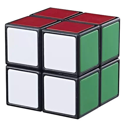
Thus, if you want to improve spatial resolution by a factor 10, you will need to perform 103 = 1000 times as many calculations. That is the difference of sub-dividing the ocean into blocks of water with a side length of 10m rather than 100m.
Temporal resolution
But wait, there is more. A computer model simulating the behaviour of some complex natural system does so by calculating its state step-by-step in some intervals of time.
One may liken it to taking a series of snapshots which together comprise a movie where movements become apparent. Question is how small the increments in time need to be in order for the model to render a reasonable realistic rendition of reality.
Consider again the flow diagram in Figure 1, representing how nitrogen flows through an aquatic ecosystem. Nitrogen and phosphorus are essential nutrients for plankton. As such, they are also termed “limiting” because the lack of either will keep plankton growth at bay—something that is often desired and virtually always in lake restoration.
Figure 1. A diagram showing “A nitrogen-based model of plankton dynamics in the oceanic mixed layer” by Fasham, M. J. (et al, 1990). The connecting arrows indicate flows of material between these components, driven by processes such as primary production, grazing and remineralisation. Closed-headed arrows indicate flows of material that remain within the model ecosystem; open-headed arrows indicate flows of material out of the modelled domain—for instance, below the ocean’s upper mixed layer.
Each of these boxes in the diagram represent compartments, which can hold the nutrient for some time. Some amount of nutrient will be bound in the biomass of phytoplankton (one compartment) for some time before it flows to another, i.e. the compartment representing zooplankton and so on.
At this point, it should hopefully be apparent how these flows are mathematically analogous to our example with the car travelling from A to B—only in this case, we are looking into the movements of nutrients between the compartments comprising the ecosystem.
Decide what is important
The flows between these compartments may have different magnitude and happen over different time scales, so they are not equally important. We can keep adding compartments and flows to our model, which will make it more realistic but also more complex.
We may also choose to do calculations in still smaller increments of time, which will also add accuracy. Only, it should be obvious that every time we make our model more complex, adding more details or making the resolution finer, it often comes with a huge penalty in terms of computational power required.
Make some choices
To make models of any practical use, something has to give. This is where we start cutting out the less important factors, settling for a cruder but more practical picture. We comb over our models and weed out the more unlikely scenarios, or we simply restrict the model to only apply to certain circumstances.
In other words, we choose not to run simulations for every possible combination of variables, as there would be too many scenarios to consider. So, we leave some out.
Mind the assumptions
This is where the concept of underlying assumptions comes into the picture. These assumptions are quite often ignored in debates or when models are criticised. But the limitations within which the model is operated are as important as how the model itself has been formulated.
Models have some limited applicability and accuracy, which should always be taken into consideration. When they are not, that is where and when things can go awry, if decisions are made on this basis.
On a related note, this may go some way to explain why divers, on some occasions, end up getting bent, despite following protocol and staying well inside decompression limits.
As sophisticated as our dive instruments have become, most of us do not stand a chance in understanding the algorithms used. But we can all appreciate that they will never be perfect, resting on assumptions and equations that hold true in most cases, while there may be rare instances, say, unusual combinations of factors, where they do not. ■


")